How to Create a Pivot Table in Excel: A Step-by-Step Tutorial

The pivot table is one of Microsoft Excel's most powerful — and intimidating — functions. Powerful because it can help you summarize and make sense of large data sets. Intimidating because you're not exactly an Excel expert, and pivot tables have always had a reputation for being complicated.

The good news: Learning how to create a pivot table in Excel is much easier than you might've been led to believe.

But before we walk you through the process of creating one, let's take a step back and make sure you understand exactly what a pivot table is, and why you might need to use one.

In other words, pivot tables extract meaning from that seemingly endless jumble of numbers on your screen. And more specifically, it lets you group your data in different ways so you can draw helpful conclusions more easily.

The "pivot" part of a pivot table stems from the fact that you can rotate (or pivot) the data in the table to view it from a different perspective. To be clear, you're not adding to, subtracting from, or otherwise changing your data when you make a pivot. Instead, you're simply reorganizing the data so you can reveal useful information from it.

What are pivot tables used for?

If you're still feeling a bit confused about what pivot tables actually do, don't worry. This is one of those technologies that are much easier to understand once you've seen it in action.

The purpose of pivot tables is to offer user-friendly ways to quickly summarize large amounts of data. They can be used to better understand, display, and analyze numerical data in detail — and can help identify and answer unanticipated questions surrounding it.

Here are seven hypothetical scenarios where a pivot table could be a solution:

1. Comparing sales totals of different products.

Say you have a worksheet that contains monthly sales data for three different products — product 1, product 2, and product 3 — and you want to figure out which of the three has been bringing in the most bucks. You could, of course, look through the worksheet and manually add the corresponding sales figure to a running total every time product 1 appears. You could then do the same for product 2, and product 3 until you have totals for all of them. Piece of cake, right?

Now, imagine your monthly sales worksheet has thousands and thousands of rows. Manually sorting through them all could take a lifetime. Using a pivot table, you can automatically aggregate all of the sales figures for product 1, product 2, and product 3 — and calculate their respective sums — in less than a minute.

2. Showing product sales as percentages of total sales.

Pivot tables naturally show the totals of each row or column when you create them. But that's not the only figure you can automatically produce.

Let's say you entered quarterly sales numbers for three separate products into an Excel sheet and turned this data into a pivot table. The table would automatically give you three totals at the bottom of each column — having added up each product's quarterly sales. But what if you wanted to find the percentage these product sales contributed to all company sales, rather than just those products' sales totals?

With a pivot table, you can configure each column to give you the column's percentage of all three column totals, instead of just the column total. If three product sales totaled $200,000 in sales, for example, and the first product made $45,000, you can edit a pivot table to instead say this product contributed 22.5% of all company sales.

To show product sales as percentages of total sales in a pivot table, simply right-click the cell carrying a sales total and select Show Values As > % of Grand Total.

3. Combining duplicate data.

In this scenario, you've just completed a blog redesign and had to update a bunch of URLs. Unfortunately, your blog reporting software didn't handle it very well and ended up splitting the "view" metrics for single posts between two different URLs. So in your spreadsheet, you have two separate instances of each individual blog post. To get accurate data, you need to combine the view totals for each of these duplicates.

That's where the pivot table comes into play. Instead of having to manually search for and combine all the metrics from the duplicates, you can summarize your data (via pivot table) by blog post title, and voilà: the view metrics from those duplicate posts will be aggregated automatically.

4. Getting an employee headcount for separate departments.

Pivot tables are helpful for automatically calculating things that you can't easily find in a basic Excel table. One of those things is counting rows that all have something in common.

If you have a list of employees in an Excel sheet, for instance, and next to the employees' names are the respective departments they belong to, you can create a pivot table from this data that shows you each department name and the number of employees that belong to those departments. The pivot table effectively eliminates your task of sorting the Excel sheet by department name and counting each row manually.

5. Adding default values to empty cells.

Not every dataset you enter into Excel will populate every cell. If you're waiting for new data to come in before entering it into Excel, you might have lots of empty cells that look confusing or need further explanation when showing this data to your manager. That's where pivot tables come in.

You can easily customize a pivot table to fill empty cells with a default value, such as $0, or TBD (for "to be determined"). For large tables of data, being able to tag these cells quickly is a useful feature when many people are reviewing the same sheet.

To automatically format the empty cells of your pivot table, right-click your table and click PivotTable Options. In the window that appears, check the box labeled Empty Cells As and enter what you'd like displayed when a cell has no other value.

How to Create a Pivot Table

1. Enter your data into a range of rows and columns.
2. Sort your data by a specific attribute.
3. Highlight your cells to create your pivot table.
4. Drag and drop a field into the "Row Labels" area.
5. Drag and drop a field into the "Values" area.
6. Fine-tune your calculations.

Now that you have a better sense of what pivot tables can be used for, let's get into the nitty-gritty of how to actually create one.

Step 1. Enter your data into a range of rows and columns.

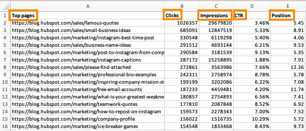
Every pivot table in Excel starts with a basic Excel table, where all your data is housed. To create this table, simply enter your values into a specific set of rows and columns. Use the topmost row or the topmost column to categorize your values by what they represent.

For example, to create an Excel table of blog post performance data, you might have a column listing each "Top Pages," a column listing each URL's "Clicks," a column listing each post's "Impressions," and so on. (We'll be using that example in the steps that follow.)

Step 2. Sort your data by a specific attribute.

When you have all the data you want entered into your Excel sheet, you'll want to sort this data in some way so it's easier to manage once you turn it into a pivot table.

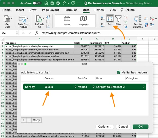
To sort your data, click the Data tab in the top navigation bar and select the Sort icon underneath it. In the window that appears, you can opt to sort your data by any column you want and in any order.

For example, to sort your Excel sheet by "Views to Date," select this column title under Column and then select whether you want to order your posts from smallest to largest, or from largest to smallest.

Select OK on the bottom-right of the Sort window, and you'll successfully reorder each row of your Excel sheet by the number of views each blog post has received.

Step 3. Highlight your cells to create your pivot table.

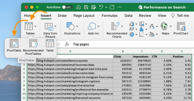
Once you've entered data into your Excel worksheet, and sorted it to your liking, highlight the cells you'd like to summarize in a pivot table. Click Insert along the top navigation, and select the PivotTable icon. You can also click anywhere in your worksheet, select "PivotTable," and manually enter the range of cells you'd like included in the PivotTable.

This will open an option box where, in addition to setting your cell range, you can select whether or not to launch this pivot table in a new worksheet or keep it in the existing worksheet. If you open a new sheet, you can navigate to and away from it at the bottom of your Excel workbook. Once you've chosen, click OK.

Alternatively, you can highlight your cells, select Recommended PivotTables to the right of the PivotTable icon, and open a pivot table with pre-set suggestions for how to organize each row and column.

Note: If you're using an earlier version of Excel, "PivotTables" may be under Tables or Data along the top navigation, rather than "Insert." In Google Sheets, you can create pivot tables from the Data dropdown along the top navigation.

Step 4. Drag and drop a field into the "Row Labels" area.

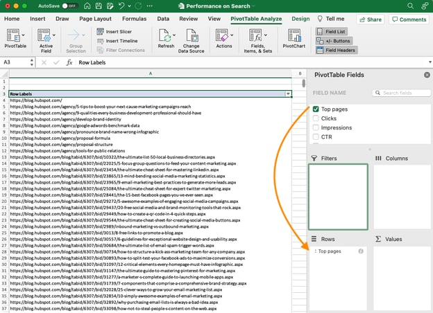
After you've completed Step 3, Excel will create a blank pivot table for you. Your next step is to drag and drop a field — labeled according to the names of the columns in your spreadsheet — into the Row Labels area. This will determine what unique identifier — blog post title, product name, and so on — the pivot table will organize your data by.

For example, let's say you want to organize a bunch of blogging data by post title. To do that, you'd simply click and drag the “Top pages” field to the "Row Labels" area.

Note: Your pivot table may look different depending on which version of Excel you're working with. However, the general principles remain the same.

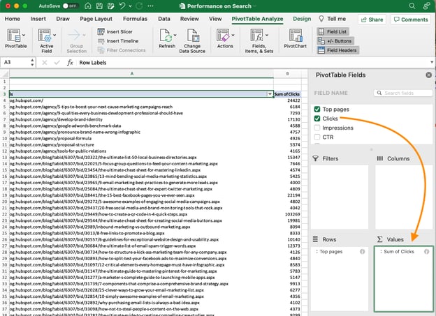
Step 5. Drag and drop a field into the "Values" area.

Once you've established what you're going to organize your data by, your next step is to add in some values by dragging a field into the Values area.

Sticking with the blogging data example, let's say you want to summarize blog post views by title. To do this, you'd simply drag the "Views" field into the Values area.

Step 6. Fine-tune your calculations.

The sum of a particular value will be calculated by default, but you can easily change this to something like average, maximum, or minimum depending on what you want to calculate.

On a Mac, you can do this by clicking on the small i next to a value in the "Values" area, selecting the option you want, and clicking "OK." Once you’ve made your selection, your pivot table will be updated accordingly.

If you're using a PC, you'll need to click on the small upside-down triangle next to your value and select Value Field Settings to access the menu.

When you’ve categorized your data to your liking, save your work and use it as you please.

Digging Deeper With Pivot Tables

You've now learned the basics of pivot table creation in Excel. With this understanding, you can figure out what you need from your pivot table and find the solutions you’re looking for.

For example, you may notice that the data in your pivot table isn't sorted the way you'd like. If this is the case, Excel's Sort function can help you out. Alternatively, you may need to incorporate data from another source into your reporting, in which case the VLOOKUP function could come in handy.

Editor's note: This post was originally published in December 2018 and has been updated for comprehensiveness.

How to Create a Pivot Table in Excel: A Step-by-Step Tutorial was originally posted by Local Sign Company Irvine, Ca. https://goo.gl/4NmUQV https://goo.gl/bQ1zHR http://www.pearltrees.com/anaheimsigns