Friday, February 18, 2022

What Are Brand Assets? 6 Examples to Inspire You

All companies that want to attract customers and stand out against competitors need strong brand assets. These elements help build an identity, maintain consistency, and create trust. Considering that trust is the second most important factor in buying from a new brand, it's essential for companies to design brand assets that highlight their values, strengths, offerings, and identities.

Brand assets let you create customer touchpoints that are immediately recognizable. Think of Amazon packaging, the Pixar lamp, or Apple's minimalist design.

But branding assets aren't simply logos and slogans. They're the combination of several elements that come together to create a unique, distinguishable identity. If well-designed, brand assets can build brand awareness, increase marketing ROI, create customer loyalty, and give you a competitive edge in the market.

Any company can develop distinct assets that draw in customers and increase sales conversations. To start, let's walk through the basics of brand assets before jumping into examples that show you how to leverage these essential branding elements.

What are Brand Assets?

Brand assets are recognizable elements that embody a company's identity. From logos and typography to taglines, brand assets make it easy to identify a business, help it stand out from competitors, and cue customer associations.

Examples of brand assetsBrand assets can include the following elements:

  • Brand name
  • Logo
  • Color palette
  • Packaging
  • Slogans or taglines
  • Songs or sounds
  • Brand guidelines
  • Mascots
  • Typography
  • Design elements
  • Voice and tone
  • Videos

Well-designed brand assets can help you deliver a consistent, unified experience and bring your business to the top of customers' minds. But it should never be mistaken for a competitor's brand. You want every element to reflect your company so it's immediately recognizable. If you can do that, your assets will work well with one another to build your unique brand identity.

Every company has different needs and thus, different assets. For some, a mascot may be more important than packaging. But all businesses must have a few essential branding assets to distinguish themselves from competitors.

Top Three Brand Assets

  • Logo: A logo is the most significant representation of a business. Research shows that people retain information better when it's paired with a relevant image, and a logo is the thing that helps customers recognize your brand and begin to build an emotional connection.
  • Color palette: Up to 90% of an initial impression is based on color alone. Considering that people form an opinion about people or products within the first 90 seconds, it's easy to see why a color palette is a top brand asset. When choosing colors, research the psychology of color to see what may resonate best with your audience.
  • Tagline: "Can you hear me now? Good." "Just do it," and "What's in your wallet?" are all famous taglines. A catchy slogan, when combined with a specific logo and color palette, can be a powerful brand asset for unifying marketing campaigns and turning your company into a household name. Just think of all the jingles you still remember from childhood!

Brand Assets Examples

When building out your company's brand assets, it can be helpful to see how other businesses stand out from the crowd. Take a look through these incredibly organized and thoughtful brand assets examples for inspiration.

Zendesk

Zendesk brand guidelines

One of my favorite collections of branding assets is Brandland, the Zendesk hub for all things brand. Not only can you discover the history and attributes behind the customer support software, but you can get information on specific assets like typography, color, and voice. It truly is a magical display.

Wistia

Wistia brand guidelines

The video hosting platform outlines its brand assets in a clear, concise way. Anyone with an interest in portraying the Wistia brand can learn how to use the logo and color palette, which comes with instructions on how to combine the two. It's simple, yet effective.

Vimeo

Vimeo grand guidelines

Compiled in a brand guideline, Vimeo shares its branding assets alongside detailed instructions on how to use them. This includes how to reference Vimeo, how to use logo color and spacing, and how to share its unique Staff Pick graphics.

Mailchimp

Mailchimp brand guidelines

Freddie is the mascot and logo for Mailchimp, which plays up the brand's offbeat humor and conversational tone. The major brand assets are shared on Mailchimp's website, as well as its content style guide — an important element for people who want to understand the brand's voice and values in an in-depth way.

HubSpot

HubSpot brand guide example

It's easy to access HubSpot brand assets through its style guide, which outlines elements like logo, color palette, tagline, graphics, and more. People can also dive into specific branding requirements so every page, product, and tool stays on-brand.

Uber

Uber brand guide

Whether someone is looking for the Uber logo or specific templates for a marketing campaign, Uber has it all in its brand playbook. The company makes it incredibly simple to understand how to use and create brand assets, which is essential for a global company that operates worldwide.

With these brand assets examples in hand, you're ready to start designing elements that showcase your identity. If you're wondering how assets play into your overall brand, look to this branding guide for tips on how to create a brand people know, love, and share.

brand consistency


What Are Brand Assets? 6 Examples to Inspire You was originally posted by Local Sign Company Irvine, Ca. https://goo.gl/4NmUQV https://goo.gl/bQ1zHR http://www.pearltrees.com/anaheimsigns

What is a Web Crawler? (In 50 Words or Less)

When it comes to technical SEO, it can be difficult to understand how it all works. But it's important to gain as much knowledge as we can to optimize our websites and reach larger audiences. One tool that plays a large role in search engine optimization is none other than the web crawler.

In this post, we’ll learn what web crawlers are, how they work, and why they should crawl your site.

Free Guide: How to Run a Technical SEO Audit

You might be wondering, "Who runs these web crawlers?"

Usually, web crawlers are operated by search engines with their own algorithms. The algorithm will tell the web crawler how to find relevant information in response to a search query.

A web spider will search (crawl) and categorize all web pages on the internet that it can find and is told to index. So you can tell a web crawler not to crawl your web page if you don't want it to be found on search engines.

To do this, you'd upload a robots.txt file. Essentially, a robots.txt file will tell a search engine how to crawl and index the pages on your site.

For example, let’s take a look at Nike.com/robots.txt.

Nike robots.txt to instruct web crawler what to index

Nike used its robot.txt file to determine which links in its website would be crawled and indexed.

Nike robots.txt file instructing web crawler to allow seven pages to be crawled and disallow three

In this portion of the file, it determined that:

  • The web crawler Baiduspider was allowed to crawl the first seven links
  • The web crawler Baiduspider was disallowed to crawl the remaining three links

This is beneficial for Nike because some pages the company has aren’t meant to be searched, and the disallowed links won’t affect its optimized pages that help them rank in search engines.

So now that we know what web crawlers are, how do they do their job? Below, let's review how web crawlers work.

A search engine's web crawler most likely won't crawl the entire internet. Rather, it will decide the importance of each web page based on factors including how many other pages link to that page, page views, and even brand authority. So, a web crawler will determine which pages to crawl, what order to crawl them in, and how often they should crawl for updates.

how web crawlers work visual chart

Image Source

For example, if you have a new web page, or changes were made on an existing page, then the web crawler will take note and update the index. Or, if you have a new web page, you can ask search engines to crawl your site.

When the web crawler is on your page, it looks at the copy and meta tags, stores that information, and indexes it for Google to sort through for keywords.

Before this entire process is started, the web crawler will look at your robots.txt file to see which pages to crawl, which is why it's so important for technical SEO.

Ultimately, when a web crawler crawls your page, it decides whether your page will show up on the search results page for a query. It's important to note that some web crawlers might behave differently than others. For example, some might use different factors when deciding which web pages are most important to crawl.

Now that we’ve gone over how web crawlers work, we’ll discuss why they should crawl your website.

Why is website crawling important?

If you want your website to rank in search engines, it needs to be indexed. Without a web crawler, your website won’t be found even if you search for over a paragraph directly taken from your website.

In a simple sense, your website cannot be found organically unless it’s crawled once.

To find and discover links on the web across search engines, you must give your site the ability to reach the audience it’s meant for by having it crawled — especially if you want to increase your organic traffic.

If the technical aspect of this is confusing, I understand. That's why HubSpot has a Website Optimization Course that puts technical topics into simple language and instructs you on how to implement your own solutions or discuss them with your web expert.

How and Why to Crawl Your Site

If your site has errors making it difficult to crawl, it could fall lower in SERP rankings. You work hard on your business and content, but – as mentioned above – no one will know how great your site is if they can’t find it online.

Luckily there are crawling tools like Screaming Frog and Deepcrawl that can shed light on the health of your website. Performing a site audit with a crawling tool can help you find common errors and identify issues such as:

  • Broken links: When links go to a page that no longer exists, it doesn’t just provide a poor user experience, but it also can harm your rankings in the SERPs.

  • Duplicate content: Duplicate content across different URLs makes it difficult for Google (or other search engines) to choose which version is the most relevant to a user’s search query. One option to remedy this is to combine them using a 301 redirect.

  • Page titles: Duplicate, missing, too long, or too short title tags all affect how your page ranks.

Web crawling tools Screaming FrogImage Source

You can’t fix problems on your site unless you know what they are. Using a web crawling tool takes the guesswork out of evaluating your site.

Types of Web Crawling Tools

There are plenty of tools on the market to choose from with various features, but they all fall into two categories:

  • Desktop: These tools are installed and stored on your computer.

  • Cloud: These tools use cloud computing and don’t have to be stored locally on your computer.

The type of tool you use will depend on your team’s needs and budget. Generally, choosing a cloud-based option will allow for more collaboration since the program won’t need to be stored on an individual’s device.

Once installed, you can set crawlers to run at a given interval and generate reports as needed.

Benefits of Using Web Crawling Tools

Having your site crawled properly is essential to SEO. In addition to diagnosing site errors, benefits of using a web crawling tool include:

1. Doesn’t Affect Site Performance

Site crawlers run in the background and won’t slow down your site when in use. They won’t interfere with your day-to-day tasks or have an effect on those browsing your site.

2. Built-in Reporting

Most crawlers have built-in reporting or analytics features and allow you to export these reports into an excel spreadsheet or other formats. This feature saves time and allows you to quickly dig into the results of your audit.

3. Utilizes Automation

A great feature of web crawlers is that you can set a cadence to have them crawl your site. This allows you to regularly track site performance without having to manually pull a crawl report each time.

Performing regular site audits with a crawling tool is a great way to ensure your site is in good health and ranking as it should.

Expand Your Reach With Web Crawling

Web crawlers are responsible for searching and indexing content online for search engines. They work by sorting and filtering through web pages so search engines understand what every web page is about. Understanding web crawlers is just one part of effective technical SEO that can improve your website’s performance significantly.

This article was originally published July 15, 2021, and has been updated for comprehensiveness.

seo audit


What is a Web Crawler? (In 50 Words or Less) was originally posted by Local Sign Company Irvine, Ca. https://goo.gl/4NmUQV https://goo.gl/bQ1zHR http://www.pearltrees.com/anaheimsigns

How to Use Excel Like a Pro: 19 Easy Excel Tips, Tricks, & Shortcuts

Sometimes, Excel seems too good to be true. All I have to do is enter a formula, and pretty much anything I'd ever need to do manually can be done automatically.

Need to merge two sheets with similar data? Excel can do it.

Need to do simple math? Excel can do it.

Need to combine information in multiple cells? Excel can do it.

In this post, I’ll go over the best tips, tricks, and shortcuts you can use right now to take your Excel game to the next level. No advanced Excel knowledge required.

Download 10 Excel Templates for Marketers [Free Kit]

What is Excel?

Microsoft Excel is powerful data visualization and analysis software, which uses spreadsheets to store, organize, and track data sets with formulas and functions. Excel is used by marketers, accountants, data analysts, and other professionals. It's part of the Microsoft Office suite of products. Alternatives include Google Sheets and Numbers. 

Find more Excel alternatives here.

Excel is primarily used for creating financial documents because of its strong computational powers. You’ll often find the software in accounting offices and teams because it allows accountants to automatically see sums, averages, and totals. With Excel, they can easily make sense of their business’ data.

While Excel is primarily known as an accounting tool, professionals in any field can use its features and formulas — especially marketers — because it can be used for tracking any type of data. It removes the need to spend hours and hours counting cells or copying and pasting performance numbers. Excel typically has a shortcut or quick fix that speeds up the process.

You can also download Excel templates below for all of your marketing needs. 

After you download the templates, it’s time to start using the software. Let’s cover the basics first.

Excel Basics

If you're just starting out with Excel, there are a few basic commands that we suggest you become familiar with. These are things like:

  • Creating a new spreadsheet from scratch.
  • Executing basic computations like adding, subtracting, multiplying, and dividing.
  • Writing and formatting column text and titles.
  • Using Excel's auto-fill features.
  • Adding or deleting single columns, rows, and spreadsheets. (Below, we'll get into how to add things like multiple columns and rows.)
  • Keeping column and row titles visible as you scroll past them in a spreadsheet, so that you know what data you're filling as you move further down the document.
  • Sorting your data in alphabetical order. 

Let's explore a few of these more in-depth. 

For instance, why does auto-fill matter? 

If you have any basic Excel knowledge, it’s likely you already know this quick trick. But to cover our bases, allow me to show you the glory of autofill. This lets you quickly fill adjacent cells with several types of data, including values, series, and formulas.

There are multiple ways to deploy this feature, but the fill handle is among the easiest. Select the cells you want to be the source, locate the fill handle in the lower-right corner of the cell, and either drag the fill handle to cover cells you want to fill or just double click:

excel autofillSimilarly, sorting is an important feature you'll want to know when organizing your data in Excel. 

Sometimes you may have a list of data that has no organization whatsoever. Maybe you exported a list of your marketing contacts or blog posts. Whatever the case may be, Excel’s sort feature will help you alphabetize any list.

Click on the data in the column you want to sort. Then click on the "Data" tab in your toolbar and look for the "Sort" option on the left. If the "A" is on top of the "Z," you can just click on that button once. If the "Z" is on top of the "A," click on the button twice. When the "A" is on top of the "Z," that means your list will be sorted in alphabetical order. However, when the "Z" is on top of the "A," that means your list will be sorted in reverse alphabetical order.

Let's explore more of the basics of Excel (along with advanced features) next. 

How to Use Excel

To use Excel, you only need to input the data into the rows and columns. And then you'll use formulas and functions to turn that data into insights. 

We're going to go over the best formulas and functions you need to know. But first, let's take a look at the types of documents you can create using the software. That way, you have an overarching understanding of how you can use Excel in your day-to-day. 

Documents You Can Create in Excel

Not sure how you can actually use Excel in your team? Here is a list of documents you can create:

  • Income Statements: You can use an Excel spreadsheet to track a company’s sales activity and financial health.
  • Balance Sheets: Balance sheets are among the most common types of documents you can create with Excel. It allows you to get a holistic view of a company’s financial standing.
  • Calendar: You can easily create a spreadsheet monthly calendar to track events or other date-sensitive information.

Here are some documents you can create specifically for marketers.

This is only a small sampling of the types of marketing and business documents you can create in Excel. We’ve created an extensive list of Excel templates you can use right now for marketing, invoicing, project management, budgeting, and more.

In the spirit of working more efficiently and avoiding tedious, manual work, here are a few Excel formulas and functions you’ll need to know.

Excel Formulas

It’s easy to get overwhelmed by the wide range of Excel formulas that you can use to make sense out of your data. If you’re just getting started using Excel, you can rely on the following formulas to carry out some complex functions — without adding to the complexity of your learning path.

  • Equal sign: Before creating any formula, you’ll need to write an equal sign (=) in the cell where you want the result to appear.
  • Addition: To add the values of two or more cells, use the + sign. Example: =C5+D3.
  • Subtraction: To subtract the values of two or more cells, use the - sign. Example: =C5-D3.
  • Multiplication: To multiply the values of two or more cells, use the * sign. Example: =C5*D3.
  • Division: To divide the values of two or more cells, use the / sign. Example: =C5/D3.

Putting all of these together, you can create a formula that adds, subtracts, multiplies, and divides all in one cell. Example: =(C5-D3)/((A5+B6)*3).

For more complex formulas, you’ll need to use parentheses around the expressions to avoid accidentally using the PEMDAS order of operations. Keep in mind that you can use plain numbers in your formulas.

Excel Functions

Excel functions automate some of the tasks you would use in a typical formula. For instance, instead of using the + sign to add up a range of cells, you’d use the SUM function. Let’s look at a few more functions that will help automate calculations and tasks.

  • SUM: The SUM function automatically adds up a range of cells or numbers. To complete a sum, you would input the starting cell and the final cell with a colon in between. Here’s what that looks like: SUM(Cell1:Cell2). Example: =SUM(C5:C30).
  • AVERAGE: The AVERAGE function averages out the values of a range of cells. The syntax is the same as the SUM function: AVERAGE(Cell1:Cell2). Example: =AVERAGE(C5:C30).
  • IF: The IF function allows you to return values based on a logical test. The syntax is as follows: IF(logical_test, value_if_true, [value_if_false]). Example: =IF(A2>B2,"Over Budget","OK").
  • VLOOKUP: The VLOOKUP function helps you search for anything on your sheet’s rows. The syntax is: VLOOKUP(lookup value, table array, column number, Approximate match (TRUE) or Exact match (FALSE)). Example: =VLOOKUP([@Attorney],tbl_Attorneys,4,FALSE).
  • INDEX: The INDEX function returns a value from within a range. The syntax is as follows: INDEX(array, row_num, [column_num]).
  • MATCH: The MATCH function looks for a certain item in a range of cells and returns the position of that item. It can be used in tandem with the INDEX function. The syntax is: MATCH(lookup_value, lookup_array, [match_type]).
  • COUNTIF: The COUNTIF function returns the number of cells that meet a certain criteria or have a certain value. The syntax is: COUNTIF(range, criteria). Example: =COUNTIF(A2:A5,"London").

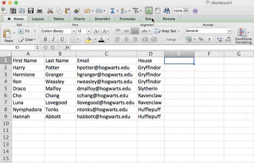
Okay, ready to get into the nitty-gritty? Let's get to it. (And to all the Harry Potter fans out there ... you're welcome in advance.)

Note: The GIFs and visuals are from a previous version of Excel. When applicable, the copy has been updated to provide instruction for users of both newer and older Excel versions.

1. Use Pivot tables to recognize and make sense of data.

Pivot tables are used to reorganize data in a spreadsheet. They won't change the data that you have, but they can sum up values and compare different information in your spreadsheet, depending on what you'd like them to do.

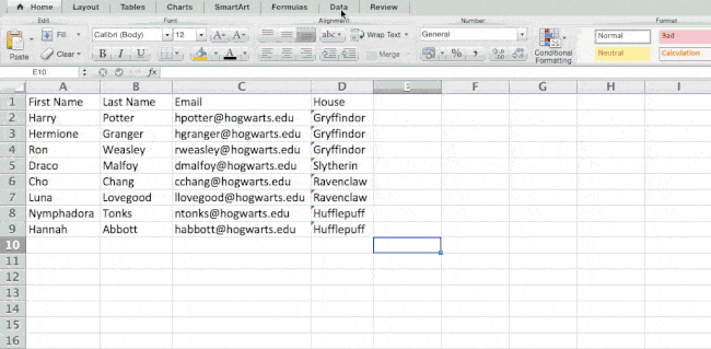
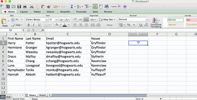
Let's take a look at an example. Let's say I want to take a look at how many people are in each house at Hogwarts. You may be thinking that I don't have too much data, but for longer data sets, this will come in handy.

To create the Pivot Table, I go to Data > Pivot Table. If you’re using the most recent version of Excel, you’d go to Insert > Pivot Table. Excel will automatically populate your Pivot Table, but you can always change around the order of the data. Then, you have four options to choose from.

  • Report Filter: This allows you to only look at certain rows in your dataset. For example, if I wanted to create a filter by house, I could choose to only include students in Gryffindor instead of all students.
  • Column Labels: These would be your headers in the dataset.
  • Row Labels: These could be your rows in the dataset. Both Row and Column labels can contain data from your columns (e.g. First Name can be dragged to either the Row or Column label — it just depends on how you want to see the data.)
  • Value: This section allows you to look at your data differently. Instead of just pulling in any numeric value, you can sum, count, average, max, min, count numbers, or do a few other manipulations with your data. In fact, by default, when you drag a field to Value, it always does a count.

Since I want to count the number of students in each house, I'll go to the Pivot table builder and drag the House column to both the Row Labels and the Values. This will sum up the number of students associated with each house.

excel pivot table creation

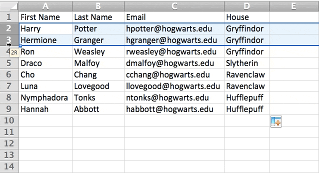
2. Add more than one row or column.

As you play around with your data, you might find you're constantly needing to add more rows and columns. Sometimes, you may even need to add hundreds of rows. Doing this one-by-one would be super tedious. Luckily, there's always an easier way.

To add multiple rows or columns in a spreadsheet, highlight the same number of preexisting rows or columns that you want to add. Then, right-click and select "Insert."

In the example below, I want to add an additional three rows. By highlighting three rows and then clicking insert, I'm able to add an additional three blank rows into my spreadsheet quickly and easily.

excel insert spaces

3. Use filters to simplify your data.

When you're looking at very large data sets, you don't usually need to be looking at every single row at the same time. Sometimes, you only want to look at data that fit into certain criteria.

That's where filters come in.

Filters allow you to pare down your data to only look at certain rows at one time. In Excel, a filter can be added to each column in your data — and from there, you can then choose which cells you want to view at once.

Let's take a look at the example below. Add a filter by clicking the Data tab and selecting "Filter." Clicking the arrow next to the column headers and you'll be able to choose whether you want your data to be organized in ascending or descending order, as well as which specific rows you want to show.

In my Harry Potter example, let's say I only want to see the students in Gryffindor. By selecting the Gryffindor filter, the other rows disappear.

excel filtersPro Tip: Copy and paste the values in the spreadsheet when a Filter is on to do additional analysis in another spreadsheet.

4. Remove duplicate data points or sets.

Larger data sets tend to have duplicate content. You may have a list of multiple contacts in a company and only want to see the number of companies you have. In situations like this, removing the duplicates comes in quite handy.

To remove your duplicates, highlight the row or column that you want to remove duplicates of. Then, go to the Data tab and select "Remove Duplicates" (which is under the Tools subheader in the older version of Excel). A pop-up will appear to confirm which data you want to work with. Select "Remove Duplicates," and you're good to go.

excel duplicates removal

You can also use this feature to remove an entire row based on a duplicate column value. So if you have three rows with Harry Potter's information and you only need to see one, then you can select the whole dataset and then remove duplicates based on email. Your resulting list will have only unique names without any duplicates.

5. Transpose rows into columns.

When you have rows of data in your spreadsheet, you might decide you actually want to transform the items in one of those rows into columns (or vice versa). It would take a lot of time to copy and paste each individual header — but what the transpose feature allows you to do is simply move your row data into columns, or the other way around.

Start by highlighting the column that you want to transpose into rows. Right-click it, and then select "Copy." Next, select the cells on your spreadsheet where you want your first row or column to begin. Right-click on the cell, and then select "Paste Special." A module will appear — at the bottom, you'll see an option to transpose. Check that box and select OK. Your column will now be transferred to a row or vice-versa.

excel transpose

On newer versions of Excel, a drop-down will appear instead of a pop-up.

Excel transpose tool in newer versions

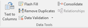
6. Split up text information between columns.

What if you want to split out information that's in one cell into two different cells? For example, maybe you want to pull out someone's company name through their email address. Or perhaps you want to separate someone's full name into a first and last name for your email marketing templates.

Thanks to Excel, both are possible. First, highlight the column that you want to split up. Next, go to the Data tab and select "Text to Columns." A module will appear with additional information.

First, you need to select either "Delimited" or "Fixed Width."

  • "Delimited" means you want to break up the column based on characters such as commas, spaces, or tabs.
  • "Fixed Width" means you want to select the exact location on all the columns that you want the split to occur.

In the example case below, let's select "Delimited" so we can separate the full name into first name and last name.

Then, it's time to choose the Delimiters. This could be a tab, semi-colon, comma, space, or something else. ("Something else" could be the "@" sign used in an email address, for example.) In our example, let's choose the space. Excel will then show you a preview of what your new columns will look like.

When you're happy with the preview, press "Next." This page will allow you to select Advanced Formats if you choose to. When you're done, click "Finish."

excel text to column

7. Use formulas for simple calculations.

In addition to doing pretty complex calculations, Excel can help you do simple arithmetic like adding, subtracting, multiplying, or dividing any of your data.

  • To add, use the + sign.
  • To subtract, use the - sign.
  • To multiply, use the * sign.
  • To divide, use the / sign.

You can also use parentheses to ensure certain calculations are done first. In the example below (10+10*10), the second and third 10 were multiplied together before adding the additional 10. However, if we made it (10+10)*10, the first and second 10 would be added together first.

Excel simple formulas in action

8. Get the average of numbers in your cells.

If you want the average of a set of numbers, you can use the formula =AVERAGE(Cell1:Cell2). If you want to sum up a column of numbers, you can use the formula =SUM(Cell1:Cell2).

9. Use conditional formatting to make cells automatically change color based on data.

Conditional formatting allows you to change a cell's color based on the information within the cell. For example, if you want to flag certain numbers that are above average or in the top 10% of the data in your spreadsheet, you can do that. If you want to color code commonalities between different rows in Excel, you can do that. This will help you quickly see information that is important to you.

To get started, highlight the group of cells you want to use conditional formatting on. Then, choose "Conditional Formatting" from the Home menu and select your logic from the dropdown. (You can also create your own rule if you want something different.) A window will pop up that prompts you to provide more information about your formatting rule. Select "OK" when you're done, and you should see your results automatically appear.

Excel conditional formatting

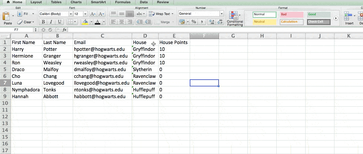
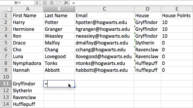
10. Use the IF Excel formula to automate certain Excel functions.

Sometimes, we don't want to count the number of times a value appears. Instead, we want to input different information into a cell if there is a corresponding cell with that information.

For example, in the situation below, I want to award ten points to everyone who belongs in the Gryffindor house. Instead of manually typing in 10's next to each Gryffindor student's name, I can use the IF Excel formula to say that if the student is in Gryffindor, then they should get ten points.

The formula is: IF(logical_test, value_if_true, [value_if_false])

Example Shown Below: =IF(D2="Gryffindor","10","0")

In general terms, the formula would be IF(Logical Test, value of true, value of false). Let's dig into each of these variables.

  • Logical_Test: The logical test is the "IF" part of the statement. In this case, the logic is D2="Gryffindor" because we want to make sure that the cell corresponding with the student says "Gryffindor." Make sure to put Gryffindor in quotation marks here.
  • Value_if_True: This is what we want the cell to show if the value is true. In this case, we want the cell to show "10" to indicate that the student was awarded the 10 points. Only use quotation marks if you want the result to be text instead of a number.
  • Value_if_False: This is what we want the cell to show if the value is false. In this case, for any student not in Gryffindor, we want the cell to show "0". Only use quotation marks if you want the result to be text instead of a number.

Excel IF formula in action

Note: In the example above, I awarded 10 points to everyone in Gryffindor. If I later wanted to sum the total number of points, I wouldn't be able to because the 10's are in quotes, thus making them text and not a number that Excel can sum.

The real power of the IF function comes when you string multiple IF statements together, or nest them. This allows you to set multiple conditions, get more specific results, and ultimately organize your data into more manageable chunks.

Ranges are one way to segment your data for better analysis. For example, you can categorize data into values that are less than 10, 11 to 50, or 51 to 100. Here's how that looks in practice: 

=IF(B3<11,“10 or less”,IF(B3<51,“11 to 50”,IF(B3<100,“51 to 100”)))

It can take some trial-and-error, but once you have the hang of it, IF formulas will become your new Excel best friend.

11. Use dollar signs to keep one cell's formula the same regardless of where it moves.

Have you ever seen a dollar sign in an Excel formula? When used in a formula, it isn't representing an American dollar; instead, it makes sure that the exact column and row are held the same even if you copy the same formula in adjacent rows.

You see, a cell reference — when you refer to cell A5 from cell C5, for example — is relative by default. In that case, you're actually referring to a cell that's five columns to the left (C minus A) and in the same row (5). This is called a relative formula. When you copy a relative formula from one cell to another, it'll adjust the values in the formula based on where it's moved. But sometimes, we want those values to stay the same no matter whether they're moved around or not — and we can do that by turning the formula into an absolute formula.

To change the relative formula (=A5+C5) into an absolute formula, we'd precede the row and column values by dollar signs, like this: (=$A$5+$C$5). (Learn more on Microsoft Office's support page here.)

12. Use the VLOOKUP function to pull data from one area of a sheet to another.

Have you ever had two sets of data on two different spreadsheets that you want to combine into a single spreadsheet?

For example, you might have a list of people's names next to their email addresses in one spreadsheet, and a list of those same people's email addresses next to their company names in the other — but you want the names, email addresses, and company names of those people to appear in one place.

I have to combine data sets like this a lot — and when I do, the VLOOKUP is my go-to formula.

Before you use the formula, though, be absolutely sure that you have at least one column that appears identically in both places. Scour your data sets to make sure the column of data you're using to combine your information is exactly the same, including no extra spaces.

The formula: =VLOOKUP(lookup value, table array, column number, Approximate match (TRUE) or Exact match (FALSE))

The formula with variables from our example below: =VLOOKUP(C2,Sheet2!A:B,2,FALSE)

In this formula, there are several variables. The following is true when you want to combine information in Sheet 1 and Sheet 2 onto Sheet 1.

  • Lookup Value: This is the identical value you have in both spreadsheets. Choose the first value in your first spreadsheet. In the example that follows, this means the first email address on the list, or cell 2 (C2).
  • Table Array: The table array is the range of columns on Sheet 2 you're going to pull your data from, including the column of data identical to your lookup value (in our example, email addresses) in Sheet 1 as well as the column of data you're trying to copy to Sheet 1. In our example, this is "Sheet2!A:B." "A" means Column A in Sheet 2, which is the column in Sheet 2 where the data identical to our lookup value (email) in Sheet 1 is listed. The "B" means Column B, which contains the information that's only available in Sheet 2 that you want to translate to Sheet 1.
  • Column Number: This tells Excel which column the new data you want to copy to Sheet 1 is located in. In our example, this would be the column that "House" is located in. "House" is the second column in our range of columns (table array), so our column number is 2. [Note: Your range can be more than two columns. For example, if there are three columns on Sheet 2 — Email, Age, and House — and you still want to bring House onto Sheet 1, you can still use a VLOOKUP. You just need to change the "2" to a "3" so it pulls back the value in the third column: =VLOOKUP(C2:Sheet2!A:C,3,false).]
  • Approximate Match (TRUE) or Exact Match (FALSE): Use FALSE to ensure you pull in only exact value matches. If you use TRUE, the function will pull in approximate matches.

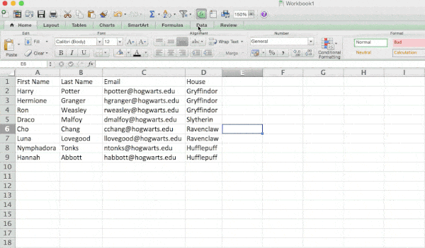
In the example below, Sheet 1 and Sheet 2 contain lists describing different information about the same people, and the common thread between the two is their email addresses. Let's say we want to combine both datasets so that all the house information from Sheet 2 translates over to Sheet 1.

Excel VLOOKUP function

So when we type in the formula =VLOOKUP(C2,Sheet2!A:B,2,FALSE), we bring all the house data into Sheet 1.

Keep in mind that VLOOKUP will only pull back values from the second sheet that are to the right of the column containing your identical data. This can lead to some limitations, which is why some people prefer to use the INDEX and MATCH functions instead.

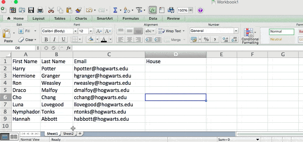
13. Use INDEX and MATCH formulas to pull data from horizontal columns.

Like VLOOKUP, the INDEX and MATCH functions pull in data from another dataset into one central location. Here are the main differences:

  • VLOOKUP is a much simpler formula. If you're working with large data sets that would require thousands of lookups, using the INDEX and MATCH function will significantly decrease load time in Excel.
  • The INDEX and MATCH formulas work right-to-left, whereas VLOOKUP formulas only work as a left-to-right lookup. In other words, if you need to do a lookup that has a lookup column to the right of the results column, then you'd have to rearrange those columns in order to do a VLOOKUP. This can be tedious with large datasets and/or lead to errors.

So if I want to combine information in Sheet 1 and Sheet 2 onto Sheet 1, but the column values in Sheets 1 and 2 aren't the same, then to do a VLOOKUP, I would need to switch around my columns. In this case, I'd choose to do an INDEX and MATCH instead.

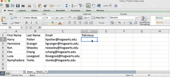
Let's look at an example. Let's say Sheet 1 contains a list of people's names and their Hogwarts email addresses, and Sheet 2 contains a list of people's email addresses and the Patronus that each student has. (For the non-Harry Potter fans out there, every witch or wizard has an animal guardian called a "Patronus" associated with him or her.) The information that lives in both sheets is the column containing email addresses, but this email address column is in different column numbers on each sheet. I'd use the INDEX and MATCH formulas instead of VLOOKUP so I wouldn't have to switch any columns around.

So what's the formula, then? The formula is actually the MATCH formula nested inside the INDEX formula. You'll see I differentiated the MATCH formula using a different color here.

The formula: =INDEX(table array, MATCH formula)

This becomes: =INDEX(table array, MATCH (lookup_value, lookup_array))

The formula with variables from our example below: =INDEX(Sheet2!A:A,(MATCH(Sheet1!C:C,Sheet2!C:C,0)))

Here are the variables:

  • Table Array: The range of columns on Sheet 2 containing the new data you want to bring over to Sheet 1. In our example, "A" means Column A, which contains the "Patronus" information for each person.
  • Lookup Value: This is the column in Sheet 1 that contains identical values in both spreadsheets. In the example that follows, this means the "email" column on Sheet 1, which is Column C. So: Sheet1!C:C.
  • Lookup Array: This is the column in Sheet 2 that contains identical values in both spreadsheets. In the example that follows, this refers to the "email" column on Sheet 2, which happens to also be Column C. So: Sheet2!C:C.

Once you have your variables straight, type in the INDEX and MATCH formulas in the top-most cell of the blank Patronus column on Sheet 1, where you want the combined information to live.

Excel INDEX and MATCH functions in action

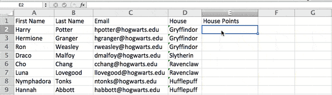
14. Use the COUNTIF function to make Excel count words or numbers in any range of cells.

Instead of manually counting how often a certain value or number appears, let Excel do the work for you. With the COUNTIF function, Excel can count the number of times a word or number appears in any range of cells.

For example, let's say I want to count the number of times the word "Gryffindor" appears in my data set.

The formula: =COUNTIF(range, criteria)

The formula with variables from our example below: =COUNTIF(D:D,"Gryffindor")

In this formula, there are several variables:

  • Range: The range that we want the formula to cover. In this case, since we're only focusing on one column, we use "D:D" to indicate that the first and last column are both D. If I were looking at columns C and D, I would use "C:D."
  • Criteria: Whatever number or piece of text you want Excel to count. Only use quotation marks if you want the result to be text instead of a number. In our example, the criteria is "Gryffindor."

Simply typing in the COUNTIF formula in any cell and pressing "Enter" will show me how many times the word "Gryffindor" appears in the dataset.

Excel COUNTIF function

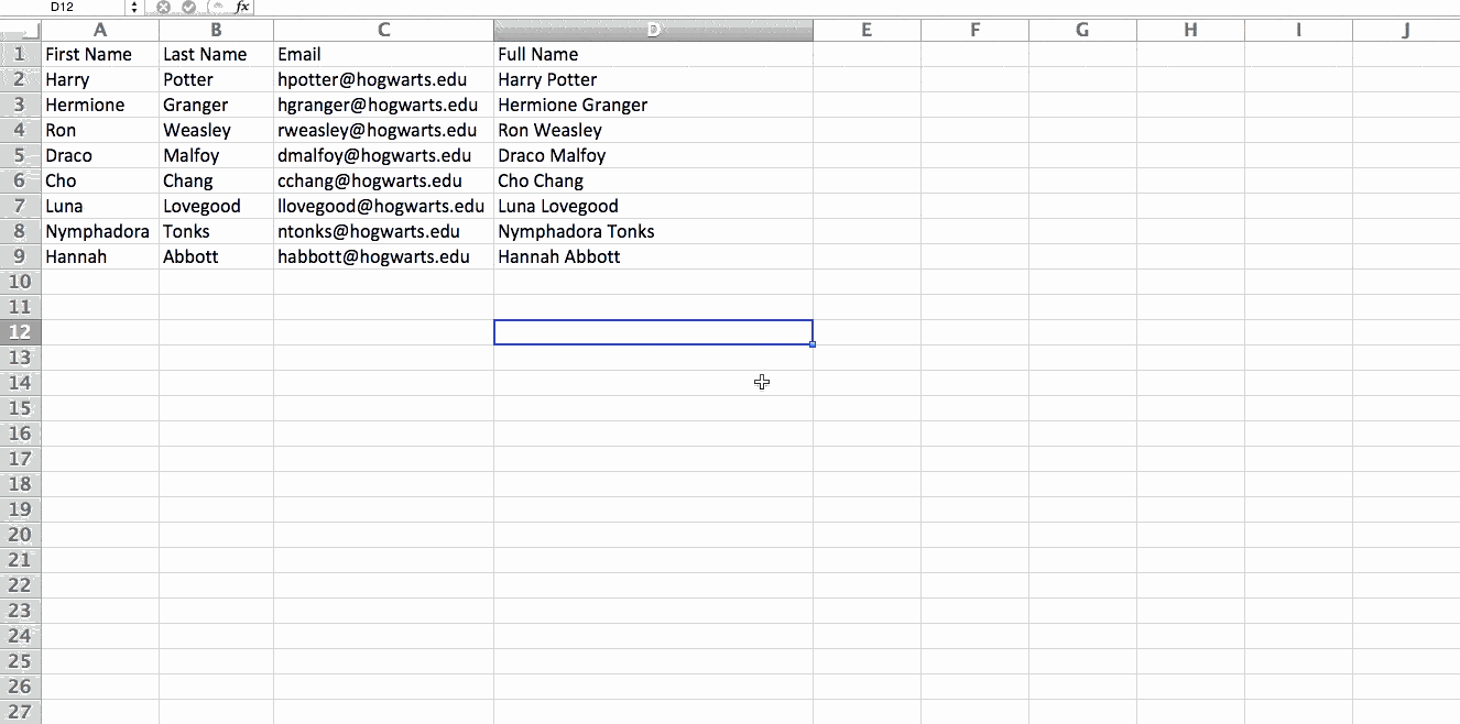
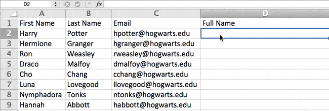
15. Combine cells using &.

Databases tend to split out data to make it as exact as possible. For example, instead of having a column that shows a person's full name, a database might have the data as a first name and then a last name in separate columns. Or, it may have a person's location separated by city, state, and zip code. In Excel, you can combine cells with different data into one cell by using the "&" sign in your function.

The formula with variables from our example below: =A2&" "&B2

Let's go through the formula together using an example. Pretend we want to combine first names and last names into full names in a single column. To do this, we'd first put our cursor in the blank cell where we want the full name to appear. Next, we'd highlight one cell that contains a first name, type in an "&" sign, and then highlight a cell with the corresponding last name.

But you're not finished — if all you type in is =A2&B2, then there will not be a space between the person's first name and last name. To add that necessary space, use the function =A2&" "&B2. The quotation marks around the space tell Excel to put a space in between the first and last name.

To make this true for multiple rows, simply drag the corner of that first cell downward as shown in the example.

Excel combination of cells

16. Add checkboxes.

If you're using an Excel sheet to track customer data and want to oversee something that isn't quantifiable, you could insert checkboxes into a column.

For example, if you're using an Excel sheet to manage your sales prospects and want to track whether you called them in the last quarter, you could have a "Called this quarter?" column and check off the cells in it when you've called the respective client.

Here's how to do it.

Highlight a cell you'd like to add checkboxes to in your spreadsheet. Then, click DEVELOPER. Then, under FORM CONTROLS, click the checkbox or the selection circle highlighted in the image below.

Excel checkboxes

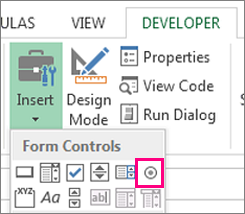
Once the box appears in the cell, copy it, highlight the cells you also want it to appear in, and then paste it.

17. Hyperlink a cell to a website.

If you're using your sheet to track social media or website metrics, it can be helpful to have a reference column with the links each row is tracking. If you add a URL directly into Excel, it should automatically be clickable. But, if you have to hyperlink words, such as a page title or the headline of a post you're tracking, here's how.

Highlight the words you want to hyperlink, then press Shift K. From there a box will pop up allowing you to place the hyperlink URL. Copy and paste the URL into this box and hit or click Enter.

If the key shortcut isn't working for any reason, you can also do this manually by highlighting the cell and clicking Insert > Hyperlink.

18. Add drop-down menus.

Sometimes, you'll be using your spreadsheet to track processes or other qualitative things. Rather than writing words into your sheet repetitively, such as "Yes", "No", "Customer Stage", "Sales Lead", or "Prospect", you can use dropdown menus to quickly mark descriptive things about your contacts or whatever you're tracking.

Here's how to add drop-downs to your cells.

Highlight the cells you want the drop-downs to be in, then click the Data menu in the top navigation and press Validation.

Excel drop-down menu option

From there, you'll see a Data Validation Settings box open. Look at the Allow options, then click Lists and select Drop-down List. Check the In-Cell dropdown button, then press OK.

19. Use the format painter. 

As you’ve probably noticed, Excel has a lot of features to make crunching numbers and analyzing your data quick and easy. But if you ever spent some time formatting a sheet to your liking, you know it can get a bit tedious.

Don’t waste time repeating the same formatting commands over and over again. Use the format painter to easily copy the formatting from one area of the worksheet to another. To do so, choose the cell you’d like to replicate, then select the format painter option (paintbrush icon) from the top toolbar.

Excel Keyboard Shortcuts 

Creating reports in Excel is time-consuming enough. How can we spend less time navigating, formatting, and selecting items in our spreadsheet? Glad you asked. There are a ton of Excel shortcuts out there, including some of our favorites listed below.

Create a New Workbook

PC: Ctrl-N | Mac: Command-N

Select Entire Row

PC: Shift-Space | Mac: Shift-Space

Select Entire Column

PC: Ctrl-Space | Mac: Control-Space

Select Rest of Column

PC: Ctrl-Shift-Down/Up | Mac: Command-Shift-Down/Up

Select Rest of Row

PC: Ctrl-Shift-Right/Left | Mac: Command-Shift-Right/Left

Add Hyperlink

PC: Ctrl-K | Mac: Command-K

Open Format Cells Window

PC: Ctrl-1 | Mac: Command-1

Autosum Selected Cells

PC: Alt-= | Mac: Command-Shift-T

Other Excel Help Resources

Use Excel to Automate Processes in Your Team

Even if you’re not an accountant, you can still use Excel to automate tasks and processes in your team. With the tips and tricks we shared in this post, you’ll be sure to use Excel to its fullest extent and get the most out of the software to grow your business.

Editor's Note: This post was originally published in August 2017 but has been updated for comprehensiveness.

excel marketing templates


How to Use Excel Like a Pro: 19 Easy Excel Tips, Tricks, &amp; Shortcuts was originally posted by Local Sign Company Irvine, Ca. https://goo.gl/4NmUQV https://goo.gl/bQ1zHR http://www.pearltrees.com/anaheimsigns

Waterfall Charts: The Marketing Graph You Need to Hit Your Goals

Last November, my husband and I were on our honeymoon in Maui. One of the main activities we wanted to do was a hiking tour near the waterfalls. We dreamt of swimming in the cascading water at sunrise.

When you hear the word “waterfall,” that’s typically what you imagine. However, today, we're going to talk about a different kind of waterfall — the waterfall chart.

→ Free Download: Free Marketing Reporting Templates [Access Now]

Waterfall charts are a data visualization resource that can help you gather and track important data such as traffic goals and lead generation. Below, let's review what a waterfall chart is, how to read one, and how to create one.

In marketing, a waterfall chart could display the number of leads, traffic sources, or blog views over a period of time. More specifically, you could use a waterfall chart to showcase how your blog traffic has increased or decreased in the last year, giving values month over month.

You could potentially use line charts, bar charts, and even bullet graphs to show this type of data. But waterfall charts have the advantage of showing your gains as they’re impacted by losses over time.

Why use a waterfall chart?

You should use a waterfall chart instead of other types of charts when trying to visualize data that experiences both gains and losses. It’s especially useful if you want to see how a loss affects a subsequent value.

waterfall chart exampleImage Source

One of the reasons that waterfall charts are effective in marketing is because they give context to the data it's reporting. Most data visualizations suffer from ignoring circumstances that result in a fall or rise in numbers, such as seasonality.

For instance, let’s say you create a waterfall chart of your Twitter followers over time. Rather than using a line graph that shows your total number of users over time, a waterfall chart shows how many you lost — and how that impacts subsequent figures.

At first glance, these charts can be difficult to read. Below, let's review how to read a waterfall chart.

How to Read a Waterfall Chart

Reading a waterfall chart will seem foreign at first if you've never done it.

However, it's important to remember that you're reading it sequentially, from left to right.

For instance, let's say you're tracking blog traffic from month to month. On the far left, you'll have the total traffic from the previous year. Then, you'll include the gains and losses month over month for the entire year. At the end of the chart, you'll see the total traffic for the year.

Here's what that looks like:

how to read a waterfall chart example

Notice how each value ends either where the previous value ended or began. In January, there was a gain of 5,000 visitors, but in February and March, there was a loss of 2,000. April’s traffic value takes that into account by starting from the -2,000 figure and going up from there.

Essentially, a waterfall chart is supposed to show you where you started and where you ended up, with details of how you got there. In this example, you can see which months gained the most traffic compared to the months that lost traffic. This could help you see seasonal adjustments, while also keeping the big picture in mind.

Now, you might be wondering, "That chart looks difficult to make. How can I make my own in Excel?" Below, we'll review the simple process of creating your own waterfall chart.

Not sure how to actually get it done? Below, we include a template and further instructions.

Bonus: You’ll also find instructions for creating waterfall charts in Google Sheets, in case that’s your preferred spreadsheet software.

Waterfall Excel Template

1. Gather your data.

Before creating your chart, you’ll need to compile the data you’d like to use.

For example, are you tracking blog traffic numbers? Or perhaps you're looking at leads generated from a certain marketing campaign? Either way, before you can create a waterfall chart, you'll need to gather your data.

2. Create a table with four columns.

For this template, we’ll track blog traffic. Create a table with four columns. The first two columns will have no headings. In cells A2 to A15, write START, then all 12 months, then END.

Waterfall chart of hypothetical blog traffic

3. Enter your data in Sheets or Excel.

Open Excel or Google Sheets, and begin manually entering your data. When you enter your data, make sure you denote the difference between positive and negative values. To denote a negative value, just add a minus sign in front of the number.

Note: all numbers in this example are arbitrary and not reflective of traffic to any blog.

Excel table for waterfall chart example.

In cell C1, write “GAIN,” and in cell D1, write “LOSS.”

From there, place your traffic numbers. How much traffic are you starting with? Write that in cell B2, next to START. Then, for each month, write how much you gained or lost.

4. Add up your values.

Add everything together, including negative values, and place them in cell B15, next to END.

5. Highlight all of your data.

Now that you have your values, highlight the table you just created.

6. Insert your waterfall chart.

If using Google Sheets, go to Insert → Chart → Waterfall chart.

This will create a waterfall chart and the Chart Editor will show up on the right-hand side. When the Chart Editor comes up, make sure that “Waterfall Chart” is selected under Chart Type.

Google Sheets Waterfall Chart selection

Waterfall chart editor in Excel.

If using Excel, go to Insert → [Waterfall chart symbol] → Waterfall.

how to create a waterfall chart in Excel

Your chart will automatically be created based on the values in our template.

7. Format your waterfall chart.

At this point, all the hard work is done. All you have to do is format your chart and make sure it looks how you want.

In Google Sheets, click on the three dots in the upper right-hand corner of the chart and hit Edit Chart. You'll get to the Chart Editor. Here, you can choose the colors of your bars, adjust your legend, or add gridlines. Most likely, the main thing you'll want to do here is to adjust your legend.

In Excel, you’ll click on the chart, then choose “Chart Design” and “Format” on the top ribbon to make the chart look the way you want it to.

Waterfall chart example with positive and negative intermediate values.

The process of creating a waterfall chart manually can be a hassle. Luckily, you can also create a waterfall chart using a dedicated dashboard tool. For example, HubSpot offers marketing dashboard and reporting software that you can use to create charts. Here's how.

How to Create a Chart in HubSpot

1. Go to Analytics Tools.

Once you log in to your portal, hover over the Reports tab and click into the Analytics Tools.

HubSpot Analytics tool can build charts for your reports.

2. Choose what you want to track.

Next, you'll choose what you want to track. Perhaps you want to analyze blog traffic like we did in the example above. Or maybe you want to review analytics for a certain campaign.

Either way, you can choose what you want to track in the Analytics Tools.

HubSpot analytics tool can build reports for marketing, sales, and service

3. Choose the chart type.

Lastly, all you have to do is choose the style chart you want. Right now, you can choose between an Area chart, Column chart, Line chart, or Combination chart. You’ll want to choose “Column,” which is closest to the waterfall chart format.

HubSpot can create various chart types.

Waterfall Analysis

To recap, here’s how to understand your waterfall chart:

A waterfall chart shows a series of negative and positive values. Each value impacts the value after it.

Example:

If one week you lose 3 leads, the next value will take that into account. If you gain 5 leads, the waterfall chart will use -3 value as a starting point, so that your ending point is a gain of 2 leads.

Each column is color-coded to distinguish positive from negative values.

Now that we have refreshed how to read and understand a waterfall chart, let’s dig into how to analyze it.

1. Examine the time ranges with the greatest losses.

Which months or weeks did you see the greatest losses? It’s important to see and understand these figures to get the most out of your chart. From there, you can troubleshoot or come up with a new strategy for those months.

2. Examine the time ranges with the greatest gains.

Conversely, look at the time ranges that saw the greatest gains. You’ll want to emulate what you did during those months — or research trends that gave you a boost during those times.

3. Examine the net change over the entire time range.

From start to end, how big of a difference did you see? Was it a positive or negative difference? Could your business have seen better results?

4. Look at week-to-week gains and losses after implementing a new strategy.

After creating a new strategy, it’ll be helpful to use a waterfall chart to see how it impacts you from week to week — whether you’re seeing more positive or negative results.

Use a waterfall chart to better analyze your performance.

To ensure you're examining the full scope of your analytics, we recommend creating a waterfall chart. It's a worthwhile data visualization tool that can help you understand your analytics sequentially. No longer do you have to rely on typical line graphs — with a waterfall chart, you’ll understand your gains and losses over time at a much more granular level.

Editor's Note: This post was originally published in May 2011 and has been updated for freshness, accuracy, and comprehensiveness.

 marketing reporting templates


Waterfall Charts: The Marketing Graph You Need to Hit Your Goals was originally posted by Local Sign Company Irvine, Ca. https://goo.gl/4NmUQV https://goo.gl/bQ1zHR http://www.pearltrees.com/anaheimsigns

Thursday, February 17, 2022

How to Improve Your Communication Skills in 5 Simple Steps

In the workplace, each employee may have their own tasks and targets, but together, you are all working toward the same end goal.

But with so many different people coming together, there’s bound to be some friction on how to implement ideas and strategies best. The key to helping your team succeed is communication.

Communication is a collaborative effort, and everyone can stand to work on their communication skills. While some workers may feel shy and won’t share their brilliant ideas, other team members may struggle to see or understand different points of view.

Download Now: 4 Free Skill Development Templates

No matter where you are with your communication skills, you can improve them with five simple steps, leading to a more collaborative and productive team.

How to Improve Communication Skills in the Workplace

5 simple ways to improve communication skillsImproving communication skills in the workplace can involve many different elements. Whether you want to be a better listener or check in with each employee, there are several ways to help your team communicate more effectively with each other. Here are five easy ways to start bettering your communication skills.

1. Be an active listener.

Are you truly listening to your team members? If you’re doodling away in a meeting, writing emails during a Zoom call, or interrupting with your own ideas or solutions, you’re not actively listening. Luckily, there are plenty of ways to improve your listening skills to ensure your co-workers feel heard.

  • Make eye contact when others are speaking.
  • Put away distractions. You can take notes, but don’t doodle, send emails, or type out texts when someone is trying to speak with you.
  • Pay attention to the other person’s tone and body language.
  • Hold your thoughts until the person is completely done speaking. When it is your turn, respond appropriately and reflect back the information just shared with you to show your attentiveness.
  • Nod and smile as appropriate while the other person is talking. If possible, try to avoid tugging at your hair, fingers, or other nearby objects.
  • Don’t plan out what to say next in your head. You can quickly become consumed by these thoughts and miss what the other person is saying.
  • Hold judgments and opinions to yourself. Avoid jumping to conclusions, and instead, let the person share everything they have to say.
  • Once the person has finished speaking, ask questions to clarify any points you are unsure about.

2. Hold effective meetings.

If you just start adding meetings to the calendar every other day, you’re probably going to have a lot of groaning and grumbling employees. Improving communication doesn’t mean hosting more meetings. The trick is to host efficient and meaningful meetings instead.

  • First thing’s first. Determine what meetings are necessary, and which ones would be better off as emails. Wasting time in unproductive meetings leaves employees with less time and energy to get their essential tasks completed.
  • Create outlines for each meeting. This helps keep everyone on topic, and you can divert back to the outline any time the conversation starts to stray.
  • Invite only the people who truly need to attend the meeting. While communication company-wide is important, it’s counterproductive to invite people to a meeting who have no need to be there. If there are a few points that pertain to someone, but they don’t need to be there for the whole meeting, invite them to attend and start with those points. Better yet, send it in an email.
  • Leave the meeting with defined action items. This helps make the meeting worthwhile.
  • Follow up with the team after the meeting. Send notes on what the meeting covered, and end with the action items expected of the team.

3. Explain the why.

When you ask an employee to start doing research for a new project or download reports, try explaining why you’re asking them to do the task. You may ask an employee to download reports for something they worked on last month.

With no explanation, they may worry that their performance was poor and they are in trouble when really you just want to apply the numbers to a new company initiative you’re working toward. 

Regardless of the task and reason, share why you are asking for certain things. This can also help avoid misunderstandings and miscommunications among the team.

4. Check-in with employees.

Even if you have an open-door policy that invites employees to speak their minds to you at any time, not everyone will take advantage of this open communication line. Some employees may feel nervous to share their thoughts or prefer to keep to themselves.

Host one-on-one meetings periodically, perhaps once a month or per quarter, to check in with each team member. Ask them about the progress on their tasks, check if they are feeling overwhelmed, and invite them to share their ideas and goals.

5. Ask for feedback.

Communication is a two-way street. In addition to leading productive meetings and checking in with employees on their tasks and project progress, you should also welcome feedback on your own performance and the company as a whole.

This can happen during one-on-one meetings, or offer regular surveys for employees to fill out. Offer an option to submit feedback anonymously as well, which can help some employees feel more comfortable speaking up.

When you receive feedback, don’t just push it to the side and forget about it. Make an action plan to work on improving your own weaknesses. If you receive feedback that applies to the company, make sure to share that information with your management as well.

Additional Options for Better Communication Skills

While these five steps are a great place to start, there are other ways to boost communication skills in the workplace. Utilize technology, such as Google Chat or Slack, to create communication channels.

If you do use an app or other communication tools, consider applying limits to when those lines are open. Constant 3 a.m. messages about a work project can lead many employees to feel burnt out if they can never switch off from work mode.

Ask your co-workers about their communication preferences, too. Surely there will be times where you have to have a meeting for everyone, but keep communication preferences in mind when you need to reach out to just one or two people. Some people retain information best when they can read it in an email, while others prefer to talk out ideas in person.

When you’re establishing effective communication among your team, make sure you include everyone. Of course, you only want to loop people into an email when it is relevant to them, but as a whole, include everyone — even if they aren’t in your section of the office or even in the same city — in your communication policies.

Finally, consider establishing an open-door policy to let employees stop by your office to discuss concerns or thoughts at any time.

Benefits of Strong Communication Skills

The benefits of improving your communication skills are seemingly endless. When everyone feels heard, there are fewer chances of tense confrontations. Plus, your team will spend less time fixing misunderstandings that happened because one person wasn’t actively listening or someone else was interrupting a meeting. That means boosted productivity and more time spent on meaningful tasks.

When your team communicates effectively across the board, you’re likely to improve the customer experience, too. Employees can meet client needs more efficiently when they can work through challenges together, and they can make sure there are minimal miscommunications that leave tasks falling through the cracks.

Better communication skills mean that every employee feels heard and more comfortable sharing their ideas. That means your team can bring more ideas to the table, which will help your company set and achieve new goals.

Communication Is Key In the Workplace

Your team is only as strong as their communication skills are. Taking time to utilize communication tools, review feedback, set meeting agendas, and conduct one-on-one sessions with employees will result in more employee engagement and productivity across the board.

Communication works both ways, so be sure to work on your own communication skills and help your team improve their communication. In the end, your company will be all the better for it.

skill improvement template


How to Improve Your Communication Skills in 5 Simple Steps was originally posted by Local Sign Company Irvine, Ca. https://goo.gl/4NmUQV https://goo.gl/bQ1zHR http://www.pearltrees.com/anaheimsigns

5 Vital Reasons to Upskill your Marketing Team

The most effective way of getting the most from your marketing team is to upskill. After all, an effective marketing team makes a business, and improving in-house skills empowers staff to grow whilst also growing the business. In-house marketing teams should not be limited to traditional activities. In the age of digital transformation, upskilling your marketing team will help push your organisation forward in line with consumer expectations.

social image state of in-housing launch blog

Find out more about which skills to provide your in-house marketing team with by reading our latest 2022 in-house marketing report:


Moving on, evidence suggests companies are not committing to upskilling their in-house teams! In fact, CXL found over 60% of marketing teams only invest around $500 on upskilling, with 20% not investing in this area at all! They are missing a trick as getting the most from your existing team is central to moving forward and keeping up with demand.

In this article we’ll look at the following key points:

  • Core skill areas for marketing teams
  • Five top reasons to upskill your marketing team
  1. Increased employee retention and satisfaction
  2. Attract better talent
  3. Higher skilled workforce
  4. Better prepared for change
  5. Return on investment (ROI)
  • How technology is enabling teams to Upskilling
  • Conclusions

Core Skill Areas for Marketing Teams

There are many different areas you can focus on when upskilling your marketing team. Some are more pressing than others. For example, a digital and tech-literate marketing team is particularly valuable to plug the recognised global skills gap. Our recent State of In-Housing Report 2022 shows where companies are already making changes to improve skill sets and where they plan to develop their digital skills in the future.

Our respondents have already invested in a range of digital marketing skill sets in the past year. Digital design and social media strategy skills topped the list, with 30% and 28% of respondents claiming they have brought in additional skill sets in these areas. Online video, media buying, and marketing automation skill sets are also high priorities, with marketing teams across different organisations already growing their skill sets in these areas.

Additional digital marketing skill sets organisations confirm they have already brought in-house:

  • Mobile design (22%)
  • Banner production (21%)
  • Copy (21%)
  • UX/UI (21%)
  • SEO (20%)
  • Content creation (19%)
  • Paid search (19%)

We also asked those surveyed to tell us about skill sets they’re hoping to bring in-house in 2022, and this delivered significantly different results. While lower priority in the last twelve months, content creation is the top priority for organisations planning to enhance their skill sets. 26% of respondents confirmed they plan to bring content creation in-house, and this is closely followed by paid search and SEO, each at 22%, which were also lower down the list of priorities in the past twelve months.

Other core skills organisations plan to bring in-house in the coming months:

  • Social media strategy (22%)
  • Banner production (22%)
  • Copy (21%)
  • Mobile design (20%)
  • Online video (19%)
  • UX/UI (19%)
  • Digital/visual design (17%)
  • Marketing automation (16%)

Many organisations have made the step to improve their in-house skill sets and upskill their marketing teams. This shows there must be benefits to this approach.

Five Reasons for Upskilling your Marketing Team

Now is the time to upskill and improve your marketing team’s credentials. The more you can manage in-house, the better value you get from your team and it also makes it easier to accelerate growth and digital change. Upskilling your marketing team comes with the following benefits.

1. Increased Employee Retention and Satisfaction

McKinsey’s research shows almost all (93%) of millennials and Generation Z employees expect learning opportunities within their job roles. Upskilling isn’t a nice extra incentive, it’s a must-have your employees expect from their employer. Upskilling helps to increase satisfaction amongst employees as they feel valued and this has a positive knock-on effect on retention, as employees are much more likely to remain with your organisations with this added benefit.

2. Attract Better Talent

Job seekers are known to apply to businesses recommended by others and a business is only likely to be recommended if they provide their teams with a great place to work and high satisfaction levels. Satisfied employees become ambassadors for your business and their networks become a talent pool for future recruitment drives. Just like your existing employees benefit from the training that comes with upskilling, new employees will be attracted by the chance to improve their skill sets when joining your organisation.

3. Higher Skilled Workforce

Identifying and filling skills gaps in your organisation is essential for future success. Upskilling programs are invaluable for adding additional skills to your workplace and giving your employees the chance to keep up with the fast pace of the digitally transforming world. Upskilling programs can be focused in the most valuable areas for your business and with your teams adequately proficient in new areas, you can be proactive in trialling new digital initiatives and techniques.

4. Better Prepared for Change

The speed at which digitisation is changing the world is forcing businesses to adapt whether they want to or not. Having the right skills within your marketing team positions you competitively and means you are ahead of the curve and ready to react to the next digital leap. By upskilling your existing team, you can benefit from their already well-known talents and push them to the levels necessary to succeed in our digital age. Your upskilling program can focus on the digital skills your organisation needs and give your team confidence in the latest technologies.

5. Return on Investment (ROI)

Yes, if you upskill your existing team it comes at a cost, but this is significantly lower than the investment necessary to hire new, skilled professionals, or utilise an outsourced service provider. The benefits of upskilling your existing marketing team delivers a return on investment in more than just financial terms. As already mentioned, you get an increased loyalty to your business and better employee retention too. It is an effective way of both ensuring your company benefits from the latest, vital skill sets and giving employees an additional incentive to remain with your organisation.

Upskilling your marketing team is something all organisations should view as imperative to keep up with rapidly changing consumer expectations and digitisation becoming the norm. Traditionally trained and experienced marketers are already primed to absorb and then practically put their new skills into action for the benefit of the wider organisation.

How technology is enabling teams to upskill

Technology is pivotal in successful upskilling. This is especially true as the new skills in demand tend to be digital and tech based. The right tools are giving brands even more freedom to grow and trial new initiatives and methods for expansion and development. The right technology can be the difference between financial success and a failed project. For example, a creative management platform (CMP), helps businesses to save money and reduce time spent on producing highly effective digital advertising assets. Other technologies such as learning management systems, or dynamic project management tools can help prioritise training. They can also help your in-house team effectively develop the new digital skills they need to succeed.

Conclusion

In our State of In-Housing Report 2022 many respondents discuss the challenges that come with developing new skills at the rates required to remain competitive. However, upskilling your in-house marketing team means having a better understanding and knowledge of your company’s core values and audience. One expert from a video games brand notes that “after working on projects for all franchises, our designers can easily begin working on a project without a lengthy onboarding process…the knowledge sharing, internally, is very easy and efficient.”

Investing in your team helps both the business and their individual development. Providing them with adequate training to upskill is one essential part of the process. You also need the right tools for success. Contact us today to see how our platform can be a valuable component of your in-house marketing upskilling strategy.

The post 5 Vital Reasons to Upskill your Marketing Team appeared first on Bannerflow.


5 Vital Reasons to Upskill your Marketing Team was originally posted by Local Sign Company Irvine, Ca. https://goo.gl/4NmUQV https://goo.gl/bQ1zHR http://www.pearltrees.com/anaheimsigns